A procedural landscape can start with a function of two variables: given a horizontal coordinate (x,z), it returns a height y. This abstraction allows generating mountains without modeling them vertex by vertex, but a noise function is not yet a renderable terrain. Between the feature and the image there is a sequence of decisions: sampling, triangulation, normals, spatial continuity, detail selection and communication with the GPU.
This article develops the ruido → campo de alturas → malla → chunks → LOD → render walkthrough, with emphasis on its mathematical invariants and engineering tradeoffs. A 3D engine or demo is not built; The proposed experiments are pending execution and no FPS figures are presented. The main reference for detail processing is Terrain Rendering Using GPU-Based Geometry Clipmaps, de Asirvatham y Hoppe.
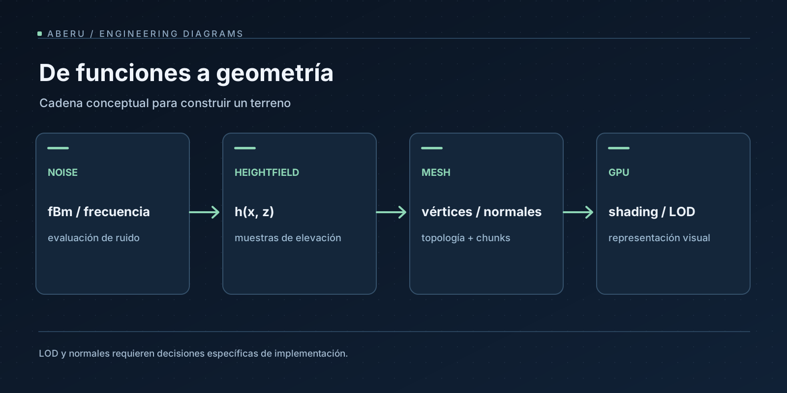
1. The promise and limit of a h(x,z) function
We define a terrain as a surface:
T(x, z) = (x, h(x, z), z)
For a point on the horizontal plane there exists a single height. This model is called heightfield or heightmap when discretized. It is efficient because it requires storing a magnitude per sample and a regular triangulation, but it has a geometric limit: it cannot represent a cave or a cantilever where there are several heights for the same position (x,z). For these cases, it would be necessary to change the representation, for example to a volumetric field and another surface extraction technique.
A procedural height normally depends on a seed s, a position in global coordinates, a set of parameters θ and the version of the algorithm:
h(x, z) = Height(s, x, z, θ, algorithm_version)
Determinism means that identical inputs and rules produce the same result within the guarantees of the implementation. Seed alone does not guarantee reproducibility if the algorithm, order of operations, data types, or floating point behavior between CPU and GPU change. To persist large worlds you must also set function version and coordinate conventions.
2. Value noise, gradient noise and why they are not the same
A distribution of independent random numbers per cell produces a visually rough surface, with no spatial correlation. To obtain connected shapes we need noise that varies smoothly in space.
Value noise: A deterministic pseudo-random value is assigned to each integer point of a grid and interpolated between corners. It is simple and pedagogical. Linear interpolation produces abrupt changes in slope at some boundaries; Smooth transition functions improve continuity of derivatives.
Gradient noise (Perlin):agradient vector is assigned to each integer vertex. At any point we calculate dot products between gradients and displacements towards the corners, and we interpolate them. It is not the same as interpolating random values. The enhanced classic fade function 6t⁵ − 15t⁴ + 10t³ has convenient derivatives at cell ends.
Simplex noise: uses another partition of space and another evaluation pattern; it is useful to understand it as an alternative to gradient noise, not as a word interchangeable with Perlin. Claims about patents, implementation licenses, and performance should be verified for the specific algorithm and library, not inferred from the generic name.
The The Book of Shaders, capítulos de ruido source allows you to inspect how interpolation and gradients transform discrete features into continuous textures. For a real engine, choosing an implementation depends on API stability, reproducibility, licensing requirements, and evaluation profile.
A noise function that respects negative coordinates
The next snippet is value noise 2D, deliberately different from Perlin. Produces deterministic samples on an infinite grid of integer coordinates, using a 32-bit hash with JavaScript integer operations and quintic interpolation. It is included as a verifiable piece of mathematics, not as a complete terrain generator.
function lattice(ix: number, iz: number, seed: number): number {
  let h = (Math.imul(ix, 374761393) ^ Math.imul(iz, 668265263) ^ seed) | 0;
  h = Math.imul(h ^ (h >>> 13), 1274126177);
  h ^= h >>> 16;
  return ((h >>> 0) / 0xffffffff) * 2 - 1;
}

const fade = (t: number): number => t * t * t * (t * (t * 6 - 15) + 10);
const mix = (a: number, b: number, t: number): number => a + (b - a) * t;

function valueNoise(x: number, z: number, seed: number): number {
  const ix = Math.floor(x), iz = Math.floor(z);
  const tx = fade(x - ix), tz = fade(z - iz);
  const a = mix(lattice(ix, iz, seed), lattice(ix + 1, iz, seed), tx);
  const b = mix(lattice(ix, iz + 1, seed), lattice(ix + 1, iz + 1, seed), tx);
  return mix(a, b, tz);
}
Using Math.floor, not truncation towards zero, avoids artificial discontinuities when crossing negative coordinates. This hash uses 32-bit integers and a normalization to approximate [-1,1]; It is not cryptographic nor does it claim perfect statistical distribution. For strict tests of equality between CPU and shaders, the same integer, rounding and formatting algorithm must be compared on both platforms.
3. fBm: superimposing scales is not equivalent to simulating geology
The so-called fractal Brownian motion in graphics is usually implemented as the sum of several octaves of noise with increasing frequencies and decreasing amplitudes:
fBm(x, z) = Σ[k=0..K−1] a_k · noise(f_k x, f_k z)

f_k = f_0 · lacunarity^k

a_k = a_0 · persistence^k
Lacunarity controls how much the frequency increases; persistence, how long the amplitude of each scale survives. If |noise| ≤ 1, we can set the |fBm| ≤ Σ|a_k| bound and normalize by dividing by that sum when it is positive. This method gives an amplitude bound, it does not force the distribution of the result to be uniform nor does it guarantee that it reaches the extremes -1 and +1.
function fbm(x: number, z: number, seed: number, octaves = 5): number {
  let amplitude = 1, frequency = 1, total = 0, norm = 0;
  for (let octave = 0; octave < octaves; octave++) {
    total += amplitude * valueNoise(x * frequency, z * frequency, seed + octave);
    norm += amplitude;
    amplitude *= 0.5;
    frequency *= 2;
  }
  return norm > 0 ? total / norm : 0;
}
A function of type ridge transforms absolute values to accentuate ridges; domain warping uses other fields to warp input coordinates and break obvious alignments. They are operations of visual synthesis, not models of hydraulic erosion, tectonics or sedimentation. Adding octaves does not “increase realism” by definition: it can create high-frequency noise that the mesh cannot represent.
Aliasing and resolution
If the spatial spacing of the grid is Δ, the highest frequency representable in one dimension should not approximately exceed the Nyquist frequency 1/(2Δ) in cycles per unit. Higher octaves can alias and produce patterns that change as you move the camera or reduce the LOD. A robust generation filters or removes unrepresentable frequencies at each level, rather than evaluating all octaves identically at all resolutions.
4. From the height field to triangles
A chunk of N × N samples contains (N−1) × (N−1) square cells. If we divide each cell into two triangles, we obtain exactly:
vértices   = N²
triángulos = 2(N−1)²
índices    = 6(N−1)²
For N = 65, that is equivalent to 4.225 vertices, 8.192 triangles, and 24.576 indices. These figures are mathematical counts, not a run benchmark. If vertices are shared through an index buffer, we avoid repeating positions in each triangle; The choice between 16 and 32 bit indexes depends on the number of indexable vertices and the buffer design.
A local vertex (i,j) is placed in world coordinates using a global origin (X0, Z0) and the sampling step Δ:
x = X0 + iΔ
z = Z0 + jΔ
y = h(x,z)
The order of indices determines the orientation of each triangle (winding). If the system uses a vertical Y axis and surfaces face up, we must maintain the same order of triangles so that back-face culling does not erase entire patches. Never deduce the orientation simply from the name of the axes: it depends on how the indices are constructed and the camera convention.
5. Normal: heights do not contain lighting
For T(x,z) = (x,h(x,z),z), two tangent vectors are (1, h_x, 0) and (0, h_z, 1). With the orientation pointing upward, a normal is proportional to:
n(x,z) = normalize(−∂h/∂x, 1, −∂h/∂z)
We can approximate both derivatives by central differences, using heights on both sides of the point. In flat areas h_x = h_z = 0, so n = (0,1,0). It is a simple and useful test case. For a chunk edge, we should not compute the derivative with missing samples and trust that the neighboring chunk will do exactly the same. Additional global samples or a shared system of normals must be consulted.
If normals are averaged from triangles, the result depends on the triangle chosen, its area, and the available neighbors. A continuous height function can produce visible lighting seams even with perfectly coincident positions if each chunk averages its normals independently.
UV coordinates are usually derived from global or local x,z depending on the texture. Local UV resets in each chunk can introduce obvious discontinuities in repeated materials. Choosing global UVs avoids certain seams, but in very large worlds it also requires managing precision and sampling scales.
6. Chunks: the boundary must be a mathematical identity
Suppose that each chunk covers M intervals of width Δ, therefore it has M+1 samples per side. For a chunk index (cx, cz) and local sample (i,j) we define:
x_global = (cx·M + i)·Δ
z_global = (cz·M + j)·Δ
The right edge of chunk cx uses i = M; the left border of cx+1 uses i = 0. Both produce exactly the same algebraic coordinates. If we calculate h using the same global deterministic function, we obtain matching heights except for possible rounding differences due to the order of operations.
That’s why the example above calculates the entire global index first and then scales: it allows shared samples to be compared unambiguously. The seed belongs to the world, not the chunk. Giving each chunk a different seed without guaranteeing continuity causes steps on the edge even though each individual texture appears smooth.
The same principle must be maintained with negative coordinates. A world with chamber left of the origin has chunks with negative indices; dividing by M and truncating towards zero can assign a position to the wrong chunk. The correct convention for partitioning in negative coordinates depends on floor, not an accidental integer cast.
Three types of sewing
**Geometric:**shared positions do not match; a real crack appears.**Shading:**equal but normal heights or different materials; a luminous line is seen.From LOD: Neighboring patches use different triangulations; one side introduces intermediate vertices that the other does not represent, creating T-junctions and possible gaps. Resolving one of these seams does not imply resolving the other two.
7. LOD: spend triangles where they have visual value
On a large terrain it is not advisable to render the same geometric density one kilometer as one meter from the camera. Level of Detail reduces geometry or sample rate in exchange for controlled visual error. Distance is a useful proxy, but the ideal criterion considers projected error on screen: a distant cliff may need more detail than a nearby plain.
Geomipmapping divides the terrain into blocks and selects one mesh version per block. It is straightforward to manage but must resolve LOD jumps; You can use stitching, skirts or geometric morphology to limit cracks and popping. Skirts hide gaps by drawing additional geometry, but they do not by themselves correct the continuity of all normals or materials.
Geometry clipmaps preserve regular grid windows nested around the camera. The scales are organized in rings; As the observer moves forward, the regions that fit into the windows are updated. Asirvatham and Hoppe explain how to represent heights through textures and reuse regular geometry to generate detail, as well as geomorphological transitions between levels. It is not “just another quadtree” nor does it in itself guarantee the absence of artifacts: updating, filtering heights and blending levels are essential parts of the method.
An LOD architecture also requires setting memory budget, criteria for loading and releasing chunks, preload margin and behavior when the generator does not finish on time. Temporarily displaying a low-resolution chunk may be preferable to blocking the render, but the transition should be explained and measured.
8. Generate heights on CPU or GPU?
There are several legitimate architectures, not a “slow CPU/fast GPU” dichotomy:
| Architecture | What does CPU calculate? | What GPU does | Main risk |
|---|---|---|---|
| CPU generated mesh | Heights, normals, indices | Rasterize mesh | Buffer and CPU increases for new chunks |
| Heightmap generated on CPU | Heights | Sample textures and move vertices | Texture transfer, format selection |
| Heightmap generated on GPU | Parameters and scheduling | Generate heights in compute/render pass and draw | Dependencies between passes and debugging |
| Noise per vertex | Coordinates, seed | Evaluate function directly in vertex shader | Repetition of calculations and CPU/GPU coherence |
WebGL2allows the use of vertex and fragment shaders, buffers, textures and framebuffers; it does not expose a general compute shader like WebGPU. It can solve numerical tasks using render-to-texture, within its formatting, capabilities, and readback limitations.WebGPU has compute passes and storage resources, but their capabilities must be tested on the actual device: using WGSL does not eliminate alignment, synchronization, or browser support requirements.
A simulation/renderer that requires collisions on the CPU may be forced to double calculate heights or read data back from the GPU; that invalidates a naive comparison that only measures shader timing. GPU transfers and waits can dominate the pipeline if synchronized every frame.
9. Large scale precision
On large worlds, adding high magnitude global positions in float32 reduces the resolution available for small offsets. It is common to save world coordinates with greater precision on the CPU and send positions relative to the camera or the local origin of the chunk to the GPU. This reduces jitter without requiring each shader operation to have 64-bit precision.
Cross-platform reproducibility has another frontier: evaluating the same octaves with different summation order, FMA, texture types and formats can produce slightly different pitches. For an application where the physics depends on height, it is advisable to define a collision source of truth and an explicit geometric tolerance, rather than assuming bitwise matching between JavaScript and WGSL.
10. A laboratory that allows us to distinguish errors
The dossier proposes an incremental construction. I would make it a test spec, not an existing demo:
- Deterministic field: same
(seed, x, z, versión)produces the same height, even with negative coordinates. - Octaves: record parameters and verify that each added frequency is representable at the sampling resolution.
- Analytical Plane: Use
h=constanteand confirm that all normals point up and heights are identical. - Mesh: check
N²,2(N−1)²counts and indices within range, in addition to winding. - Chunks: exactly compare the global coordinates and heights of shared samples of horizontal and vertical neighbors.
- LOD: inspect geometry seams and normals on pairs of different levels; log projected error and popping.
- Performance: separate CPU generation, resource load, GPU time, draw calls, visible triangles, memory and streaming latency.
In a comparison between CPU and GPU strategies we would use the same logical terrain, camera, viewport, output resolution, seed, filters and memory budget. We would record browser version, device, physical resolution, graphical limits and heating. It would not be valid to compare a CPU mesh with very detailed geometry against a GPU that renders fewer triangles and call the difference “GPU acceleration.”
Reference cases should include a plain, an analytical slope h(x,z)=ax+bz, a smooth fractal field and a pair of chunks with different LODs. An expected result should not be confused with a measurement: that two edges should coincide is a verifiable condition; To say that this implementation already brings them together without errors would require running the engine code.
11. From generated terrain to compelling world
The height alone provides silhouette. To create a credible landscape you have to compose materials by altitude and slope, humidity, temperature, erosion, drainage and vegetation. They are additional models: a snow texture applied by altitude does not simulate physical snow accumulation; a high noise pattern does not simulate geological erosion. They can be perfectly valid artistic decisions as long as they are not described as scientific validation.
The engineering conclusion is that procedural terrain is not optimized solely by accelerating noise. The mesh, LOD policy, seam continuity, precision, and data movements are often as important as the function that generates heights. The correct implementation path is to isolate these responsibilities and verify them in a reproducible way.
Readings and sources
- Arul Asirvatham y Hugues Hoppe — Terrain Rendering Using GPU-Based Geometry Clipmaps, GPU Gems 2. Nested grids, transitions and use of vertex textures.
- Hugues Hoppe — publicación y materiales del artículo de geometry clipmaps. Author’s source to review the assumptions of the approach.
- Patricio González Vivo y Jen Lowe — The Book of Shaders, ruido. Visual explanation of noise functions in shaders.
- MDN — WebGL2RenderingContext. WebGL2 pipeline contract.
- MDN — WebGPU API. Compute shaders and device limits.
Visual extensions planned: Animated comparison of noise and fBm, continuity of two chunks and LOD rings. The cover page and a conceptual diagram of the pipeline are already incorporated; there is no 3D engine or executable demo. Additional specifications continue at docs/BLOCK-08-FIGMA-SHOTLIST.md.

